On rational parametrization of circles

This is about circle parametrization. Check the google spreadsheet here

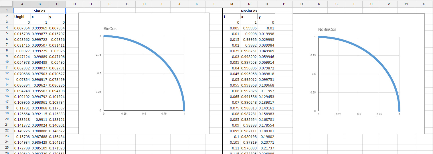
In programming and engineering in general we need to generate circles or circle like shapes. Often we need the circle points for all kinds of stuff, like drawing or object placement or procedural generation, interpolation etc. Let’s take a look at a different parametrization for the unit circle. First because we must have a common ground let us illustrate the normal (as in most used) unit circle parametrization:

$$ C(\alpha)=\begin{cases} x = \sin \alpha \ y = \cos \alpha \end{cases} , \alpha \in \mathbb{R} $$

So the circle point generation in this case is simple, we pick a resolution and iterate accordingly on $ \alpha $`.

What is the problem with this parametric representation?

The main problem is that for $\alpha \in \mathbb{Q}$ we get $(x,y) \in \mathbb{R}^2$. As we know we can’t represent $\mathbb{R}$ in computer memory because of small infinity. We just get truncated values for transcedental, irrational numbers and the process itself for getting those numbers is basically a form of never ending search. (it actually ends when we feel it’s acurate enough and it is iterative). That is why sin and cos (and actually square root and a bunch of others ) are not actually free and cost some computation.

Can we do better?

Let us try this following parametrization:

$$ C(t)=\begin{cases} x = \frac {1-t^2}{1+t^2} \ y = \frac{2t}{1+t^2} \end{cases} , t \in \mathbb{R} $$

Why should it be better?

We avoid irrational numbers by using a polynomial representation that does not expand into an infinite converging series. It should be faster and more precise.

Problems that emerge from this parametrization

• It makes a full circle only when $t \rightarrow \infty \rightarrow -\infty$ but it makes half of a circle for $t \in [-1 , 1]$
• the evolution of the generator curve is not as we expect regarding t, so we can’t actually use this where we need something expressed in angles (like representing the motion of a body using angular speed).

There are ways to fix the two problems, or at least the first one (the second one needs us to use different terminology and thought patterns in expressing problems). For the first problem we just use the circle symmetry and just reflect the points (second half of the circle is actually the first half with the x coordinate negated). We can actually do all reflections and only generate the first quadrant.

Is this faster on todays computers?

Let’s do a small performance test: We restrict our analysis on the first quadrant of the circle and generate 100000 points with both methods:

$$\begin{array}{|c|c|} \hline Function &Time (microseconds) \\ \hline C(t) & 2779 \\ \hline C(\alpha) & 7901 \\ \hline & \\ \hline C(t) & 1411 \\ \hline C(\alpha) & 3498 \\ \hline & \\ \hline C(t) & 1296 \\ \hline C(\alpha) & 3569 \\ \hline & \\ \hline C(t) & 1446 \\ \hline C(\alpha) & 3392 \\ \hline & \\ \hline C(t) & 1322 \\ \hline C(\alpha) & 3382 \\ \hline & \\ \hline C(t) & 1280 \\ \hline C(\alpha) & 3392 \\ \hline & \\ \hline C(t) & 1279 \\ \hline C(\alpha) & 3421 \\ \hline & \\ \hline C(t) & 1280 \\ \hline C(\alpha) & 3384 \\ \hline & \\ \hline C(t) & 1284 \\ \hline C(\alpha) & 3393 \\ \hline & \\ \hline C(t) & 1294 \\ \hline C(\alpha) & 3388 \\ \hline \end{array}$$

We do the same test for 10000000 points:

$$\begin{array}{|c|c|} \hline Function &Time (microseconds) \\ \hline C(t) & 128561 \\ \hline C(\alpha) & 378142 \\ \hline & \\ \hline C(t) & 129083 \\ \hline C(\alpha) & 378073 \\ \hline & \\ \hline C(t) & 128967 \\ \hline C(\alpha) & 378062 \\ \hline & \\ \hline C(t) & 128911 \\ \hline C(\alpha) & 377789 \\ \hline & \\ \hline C(t) & 129012 \\ \hline C(\alpha) & 378991 \\ \hline & \\ \hline C(t) & 128950 \\ \hline C(\alpha) & 377929 \\ \hline & \\ \hline C(t) & 128354 \\ \hline C(\alpha) & 377812 \\ \hline & \\ \hline C(t) & 129017 \\ \hline C(\alpha) & 377406 \\ \hline \end{array}$$

As we can see the t parametrization is almost 3 times faster than the angle one on my pc (I7-2600 3.40Ghz 8CPU). If you want to run the tests for yourself you may get the code here

I know most people don’t require proof, if you can see it working it’s usually enough but I’ll also provide the proof here because I like this very much:

Algebraic proof of the t parametrization

We start from this geometric interpretation:

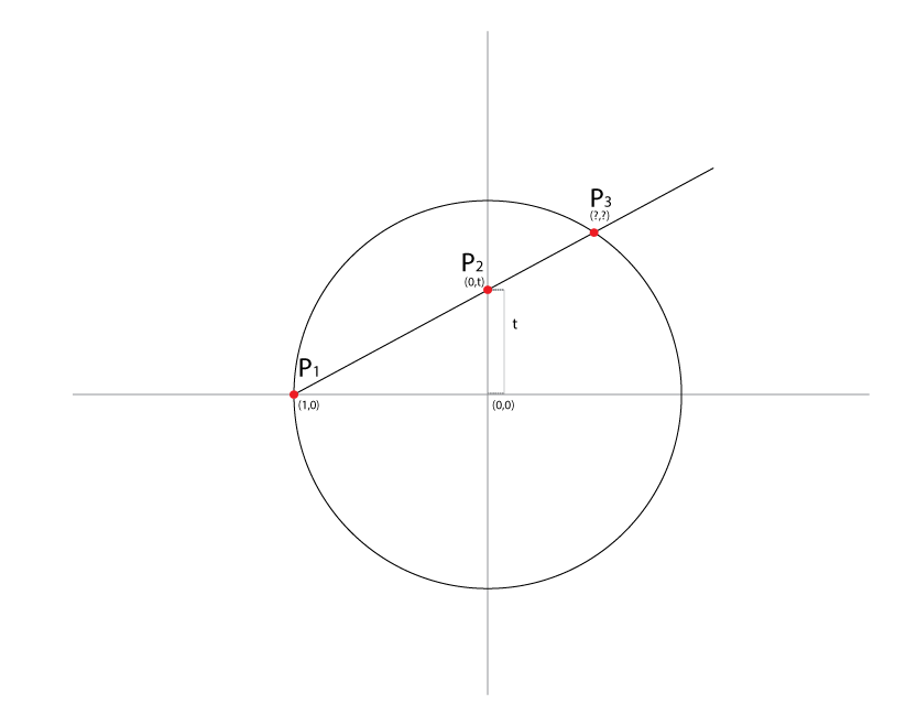
So we have this parametric line that goes through $P_1(1,0)$ and $P_2(0,t)$ and intersects our unit circle in $P_3$. If we determine the expression for $P_3$ we will have a circle parametrization in t.

We first write the line equation:$$\begin{equation} \tag{1} \label{eq} y = t(x+1) \end{equation}$$ Then we write the circle equation:$$\begin{equation} \tag{2} \label{eq2} x^2 + y^2 =1\end{equation}$$ We want to find the intersection points so we make our system out of $\eqref{eq}$ and $\eqref{eq2}$.

$$ \begin{cases} y = t(x+1) \\ x^2 + y^2 =1 \end{cases} , t \in \mathbb{R} $$

Replacing y we get:$$x^2 + t^2(x+1)^2 = 1 $$ Quadratic polynomial $$(1+t^2)x^2 + 2t^2x + t^2 -1 = 0 $$ Monic quadratic polynomial $$x^2+ \frac{2t^2}{1+t^2} x + \frac{t^2-1}{1+t^2} = 0$$ We could solve this the normal way or we can use the fact that we know for sure that a root is -1 because our circle and line meet in $P_1(-1,0)$. So we can use simple synthetic division to find the other root

$$\begin{array}{|c|c|c|} \hline 1 & \frac{2t^2}{1+t^2} & \frac{t^2 -1}{1+t^2} \\ \hline 1 & \frac{1- t^2}{1+t^2} & 0 \\ \hline \end{array}$$ so we have our factorization: $$ (x+1)(x- \frac{1-t^2}{1+t^2})$$ and then we just replace x in $\ref{eq}$ so $$P_3 \left( \frac{1-t^2}{1+t^2},\frac{2t}{1+t^2} \right) $$ then we can safely say: $$ C(t)=\begin{cases} x = \frac {1-t^2}{1+t^2} \ y = \frac{2t}{1+t^2} \end{cases} , t \in \mathbb{R} $$ We see the polynomial form returns rational output numbers for rational inputs.

This proof is geometric, algebraic and beautiful and actually relies on stereographic projection. The circle parametrization can be extended to spheres using the same methods. We can also use it to represent rotations.

Calculus proof of the t parametrization

Of course you can also go the way of calculus to get this using “The world’s sneakiest substitution undoubtedly” the tangent half-angle substitution:

Let $t = \tan \frac{\alpha}{2}$ . We know that $$\sin \alpha = 2 \sin \frac{\alpha}{2} \cos \frac{\alpha}{2} = 2t\cos^2 \frac{\alpha}{2} = \frac{2t}{sec^2 \frac{\alpha}{2}} = \frac{2t}{1+t^2}$$ Then we do the same thing for $\cos \alpha$ $$\cos \alpha = 1- 2sin^2 \frac{\alpha}{2} = 1- 2t^2 \cos^2 \frac{\alpha}{2}= 1 - \frac{2t^2}{sec^2 \frac{\alpha}{2}}= 1 - \frac{2t^2}{1+t^2} = \frac{1-t^2}{1+t^2}$$.

So that is it, we can of course derive transformation matrices from this or quaternions but I’ll stop here. Hope you enjoyed this :).

If you like rational trigonometry I wholeheartedly recommend you this book